UC Berkeley Robotics / Vision / PINN / Webots

UR5e vision-to-control pipeline.

A scientific robotics case study: object localization, neural inverse kinematics, and physics-constrained validation.

This project studies a complete simulated pick-and-place pipeline for a UR5e manipulator: a Webots camera produces object observations, a trained visual regressor estimates the target location, and a physics-informed neural network predicts the six joint angles needed to reach the object.

The core engineering question is whether a neural IK solver can be made useful for robotics by constraining it with forward kinematics, instead of treating inverse kinematics as a purely black-box regression problem.

  • Webots dataset generation
  • VGG16 visual regression
  • PINN inverse kinematics
  • Differentiable FK loss
  • IKPY baseline benchmark

01. Research framing

I redesigned this page as a technical case study: hypothesis, data, model, physics constraint, benchmark evidence, and limitations, using real project captures and data-driven figures.

Problem

Inverse kinematics is multi-solution and branch-sensitive.

A UR5e pose can correspond to several joint configurations. A naive neural regressor can average incompatible branches and output a joint vector that is numerically smooth but geometrically wrong.
Hypothesis

Forward kinematics can regularize the neural solver.

By passing predicted joints back through a differentiable FK model, the network is trained to minimize not only joint error, but also end-effector position error in Cartesian space.

Contribution

A complete Webots pipeline, not just a notebook.

The work connects dataset generation, visual target estimation, neural IK training, PyTorch physics losses, and a Webots controller benchmarked against IKPY.

Vision frames1000
Vision split800 / 200
PINN samples120k
Physics weight\(w_{phys}=20\)

02. Vision dataset and learned object localization

The vision part is based on rendered Webots observations and pixel labels. The published artefacts in the project folder show a VGG16-based visual regressor trained to predict object coordinates from images.

Dataset evidence

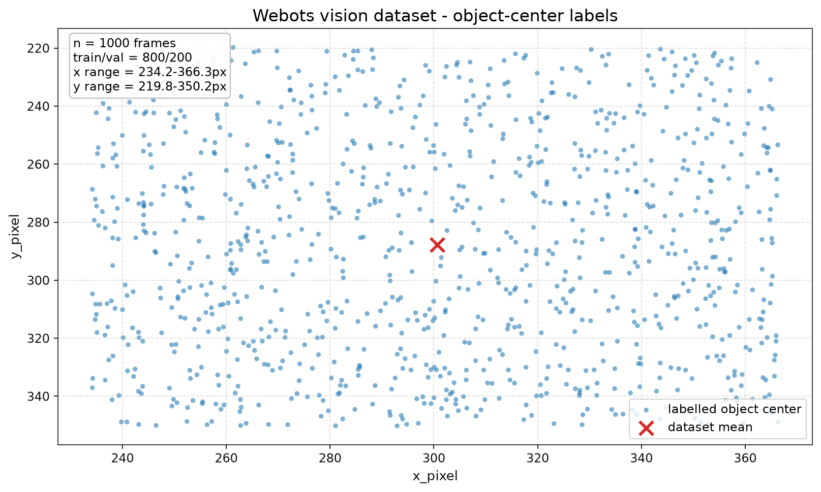
1000 Webots frames labelled with object pixel coordinates.

The dataset contains RGB frames and a CSV file with \((x_{pixel}, y_{pixel})\) targets. The model code loads the image tensor as \(1000 \times 256 \times 256 \times 3\), normalizes it, and splits it into 800 training images and 200 validation images.

  • Label range: \(x\approx234\) to \(366\) px, \(y\approx220\) to \(350\) px.
  • Supervision: each image is paired with the measured object center in the camera plane.
  • Role: convert camera evidence into a target for the downstream robot-control layer.

Vision model

Transfer learning as a coordinate regressor.

The project notebook uses a frozen VGG16 image backbone and replaces the classification head with regression layers. The output is not a class label; it is the object location in the camera image.

Input 256×256×3
Frozen backbone VGG16
Regression head 128 → 64 → 2
Output \((x,y)\)

Training setup found in the notebook

  • Backbone: VGG16 pretrained on ImageNet, no classification top.
  • Head: global average pooling, dense 128 ReLU, dense 64 ReLU, dense 2 linear.
  • Loss: MSE, metric: MAE, optimizer: Adam with learning rate \(10^{-3}\).
  • Default training path: 15 epochs, batch size 32 if no saved model is present.

03. Physics-informed inverse kinematics

The PINN maps a Cartesian target to a 6-DOF joint vector. The scientific part is the loss: the predicted joint vector is evaluated through the UR5e forward-kinematics equations during training.

1

Target point

Camera or simulation gives the desired end-effector position.

x_target = (X, Y, Z)

2

Neural IK

The MLP predicts the six UR5e joint angles.

q_pred = fθ(x_target)

3

Forward kinematics

PyTorch FK reconstructs where the predicted joints actually place the tool.

x_hat = FK(q_pred)

4

Physics residual

The residual penalizes Cartesian geometry error.

||x_hat - x_target||²

PINN objective

Supervised joint learning + physical consistency.

The implementation has two training routes: a 6-DOF dataset generated through IK sampling, and a “true physics” variant that computes the FK residual directly in PyTorch. Both keep the same principle: the joint prediction must be numerically close to data and physically coherent in Cartesian space.

$$\mathcal{L}_{total}=w_{data}\mathcal{L}_{data}+w_{phys}\mathcal{L}_{phys}$$
$$\mathcal{L}_{data}=\frac{1}{N}\sum_i\lVert \mathbf{q}^{(i)}_{pred}-\mathbf{q}^{(i)}_{IK}\rVert_2^2$$
$$\mathcal{L}_{phys}=\frac{1}{N}\sum_i\lVert FK_{UR5e}(\mathbf{q}^{(i)}_{pred})-\mathbf{x}^{(i)}_{target}\rVert_2^2$$

6-DOF PINN route

Large synthetic IK dataset.

The training script samples 120,000 candidate Cartesian targets in the UR5e workspace, keeps valid IK solutions, and trains a \(3 \rightarrow 6\) MLP with 256-neuron hidden layers, SiLU activations, batch size 256, and 60 epochs.

  • Workspace: \(x\in[0.35,0.65]\), \(y\in[-0.25,0.25]\), \(z\in[-0.25,0.10]\).
  • Split: 85% training, 15% validation.
  • Loss weights: \(w_{data}=1\), \(w_{phys}=20\).

True physics route

FK loss inside PyTorch.

A second script generates 25,000 Webots table targets and trains a 512-hidden-unit model with a differentiable UR5 FK module. It reports physics error in millimetres, joint-angle MSE, and learning-rate updates during training.

  • Table workspace: \(x\in[0.0,0.4]\), \(y\in[-0.9,-0.5]\), \(z\in[0.05,0.45]\).
  • Loss mix: \(0.1\mathcal{L}_{data}+1.0\mathcal{L}_{phys}\).
  • Output checkpoint: best physics-consistent model.

04. Training evidence and benchmark

The figures below are intentionally simple: one curve from an archived training log and one timing chart from the Webots comparison. They make the page more scientific without pretending that every experiment was already packaged like a final paper.

Training trace

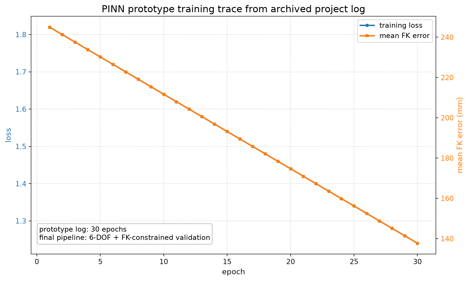
A real archived PINN run, used as development evidence.

The archived prototype log shows loss and mean FK error decreasing across 30 epochs. The later 6-DOF pipeline is more rigorous, because the code explicitly weights the physics loss and validates FK error on held-out samples.

  • Why it matters: the neural solver was not only implemented; it was trained and inspected over epochs.
  • What improved later: larger workspace sampling, 6-DOF output, validation split, and stronger physics weighting.

Webots benchmark

PINN and IKPY are compared inside the same simulation loop.

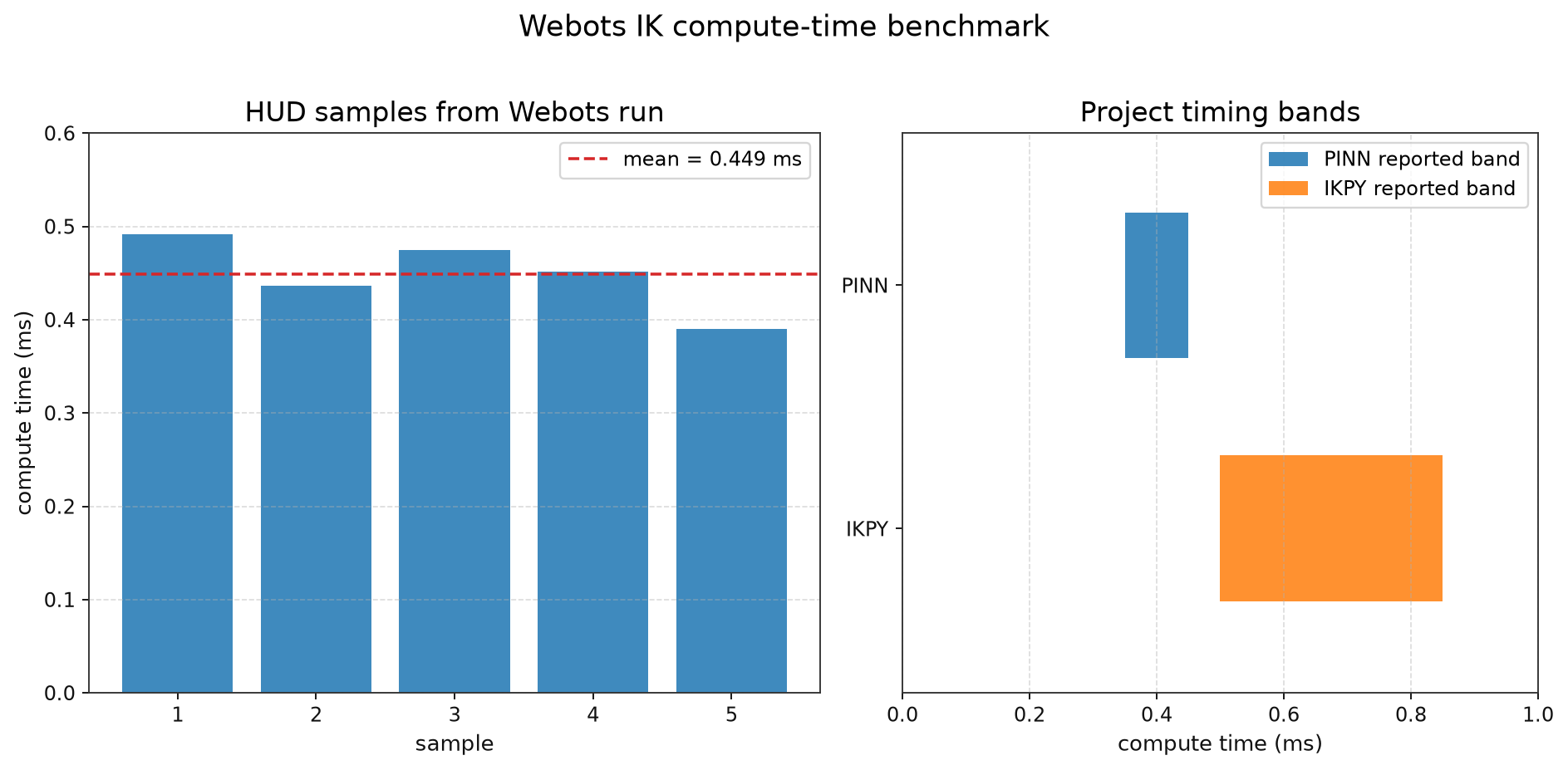
The comparative world places the neural solver beside an IKPY analytic baseline. The Webots HUD logs sub-millisecond compute times while the robot follows the target. This is the practical robotics test: not just “does the network train?”, but “can it sit inside the controller loop?”.

  • IKPY role: trusted analytic reference for reachability and timing.
  • PINN role: neural surrogate that can be regularized and benchmarked against the analytic path.
  • Observed HUD samples: around 0.39–0.49 ms for the displayed IKPY run.

05. Engineering implementation trace

These are the concrete pieces that make the project reproducible and credible as engineering work rather than a decorative AI demo.

Dataset generation Webots frames + labels

Generated camera observations and object-center coordinates for the learning pipeline.

Vision training VGG16 regression notebook

Transfer-learning model mapping \(256\times256\) RGB images to two pixel coordinates.

PINN training 6-DOF PyTorch model

MLP trained on valid IK samples with a strong forward-kinematics consistency term.

Physics model UR5e forward kinematics

Differentiable FK converts predicted joints back to Cartesian tool position.

Simulation Webots UR5e + PandaHand

Controller executes approach, grasp, lift, and placement trajectories.

Benchmark PINN vs IKPY

Analytic IK baseline kept in the loop to compare speed and qualitative behavior.

What this page now emphasizes

Data, equations, code evidence, and simulation behavior.

The project reads as a robotics study: it shows where the data comes from, how the vision model was trained, why the PINN is physically constrained, what equations define the loss, and how the solver is exercised in Webots against IKPY.

Next scientific upgrades

  • Export final 6-DOF training logs as CSV to plot validation FK error over epochs.
  • Add precision/recall/mAP curves if a YOLO detection run is later added to the folder.
  • Publish a small ablation: data loss only vs physics-informed loss.
  • Store benchmark timings over many randomized targets instead of a few HUD samples.